
实在抱歉,这周太过于忙碌,没有完成任何的要求,周末补上
- 🍨 本文为🔗365天深度学习训练营 中的学习记录博客
- 🍦 参考文章:365天深度学习训练营-第P2周:彩色识别
- 🍖 原作者:K同学啊|接辅导、项目定制
In [3]:
import torch
import torch.nn as nn
import torchvision.transforms as transforms
import torchvision
from torchvision import transforms, datasets
from sklearn.model_selection import KFold
from torch.optim.lr_scheduler import StepLR, MultiStepLR, LambdaLR, ExponentialLR, CosineAnnealingLR, ReduceLROnPlateau

import os,PIL,pathlib,random

device = torch.device("cuda" if torch.cuda.is_available() else "cpu")

device
Out[3]:
device(type='cuda')
2、导入数据
In [12]:
data_dir = './data/7-data'
# 通过Path类创建路径对象
data_dir = pathlib.Path(data_dir)
# 获取路径下所有文件路径
paths= list(data_dir.glob('*'))
# 获取所有文件夹的名字,也就是图片类别
classNames = [str(path).split("\\")[2] for path in paths] # K哥classNames中间会多一个e
classNames
Out[12]:
['Dark', 'Green', 'Light', 'Medium']
In [13]:
# 关于transforms.Compose的更多介绍可以参考:https://blog.csdn.net/qq_38251616/article/details/124878863
train_transforms = transforms.Compose([
    transforms.Resize([224, 224]),  # 将输入图片resize成统一尺寸
    # transforms.RandomHorizontalFlip(), # 随机水平翻转
    transforms.ToTensor(),          # 将PIL Image或numpy.ndarray转换为tensor,并归一化到[0,1]之间
    transforms.Normalize(           # 标准化处理-->转换为标准正太分布(高斯分布),使模型更容易收敛
        mean=[0.485, 0.456, 0.406],
        std=[0.229, 0.224, 0.225])  # 其中 mean=[0.485,0.456,0.406]与std=[0.229,0.224,0.225] 从数据集中随机抽样计算得到的。
])

test_transform = transforms.Compose([
    transforms.Resize([224, 224]),  # 将输入图片resize成统一尺寸
    transforms.ToTensor(),          # 将PIL Image或numpy.ndarray转换为tensor,并归一化到[0,1]之间
    transforms.Normalize(           # 标准化处理-->转换为标准正太分布(高斯分布),使模型更容易收敛
        mean=[0.485, 0.456, 0.406],
        std=[0.229, 0.224, 0.225])  # 其中 mean=[0.485,0.456,0.406]与std=[0.229,0.224,0.225] 从数据集中随机抽样计算得到的。
])

total_data = datasets.ImageFolder("./data/7-data/",transform=train_transforms)
total_data
Out[13]:
Dataset ImageFolder
    Number of datapoints: 1200
    Root location: ./data/7-data/
    StandardTransform
Transform: Compose(
               Resize(size=[224, 224], interpolation=bilinear, max_size=None, antialias=None)
               ToTensor()
               Normalize(mean=[0.485, 0.456, 0.406], std=[0.229, 0.224, 0.225])
           )
In [14]:
total_data.class_to_idx
Out[14]:
{'Dark': 0, 'Green': 1, 'Light': 2, 'Medium': 3}
3、划分数据集
In [15]:
train_size = int(0.8 * len(total_data))
test_size  = len(total_data) - train_size
train_dataset, test_dataset = torch.utils.data.random_split(total_data, [train_size, test_size])
train_dataset, test_dataset
Out[15]:
(<torch.utils.data.dataset.Subset at 0x1c4671c77f0>,
 <torch.utils.data.dataset.Subset at 0x1c438987c70>)
In [6]:
kf = KFold(n_splits=10,shuffle=True, random_state=42)  # 初始化KFold
for train_index , test_index in kf.split(total_dataset):  # split
    # get train, val 根据索引划分
    train_dataset = torch.utils.data.dataset.Subset(total_dataset, train_index)
    test_dataset = torch.utils.data.dataset.Subset(total_dataset, test_index)

    # package type of DataLoader
    train_loader = torch.utils.data.DataLoader(dataset=train_dataset, batch_size=batch_size, shuffle=True)
    test_loader = torch.utils.data.DataLoader(dataset=test_dataset, batch_size=batch_size, shuffle=True)

    train_loader
---------------------------------------------------------------------------
NameError                                 Traceback (most recent call last)
<ipython-input-6-4e419c68ba6d> in <module>()
      1 kf = KFold(n_splits=10,shuffle=True, random_state=42)  # 初始化KFold
----> 2for train_index , test_index in kf.split(total_dataset):  # split
      3     # get train, val 根据索引划分
      4     train_dataset = torch.utils.data.dataset.Subset(total_dataset, train_index)
      5     test_dataset = torch.utils.data.dataset.Subset(total_dataset, test_index)

NameError: name 'total_dataset' is not defined
In [16]:
batch_size = 32

train_dl = torch.utils.data.DataLoader(train_dataset,
                                       batch_size=batch_size,
                                       shuffle=True,
                                       num_workers=3)

test_dl = torch.utils.data.DataLoader(test_dataset,
                                      batch_size=batch_size,
                                      shuffle=True,
                                      num_workers=3)
In [17]:
for X, y in test_dl:
    print("Shape of X [N, C, H, W]: ", X.shape)
    print("Shape of y: ", y.shape, y.dtype)
    break
Shape of X [N, C, H, W]:  torch.Size([32, 3, 224, 224])
Shape of y:  torch.Size([32]) torch.int64
In [18]:
import torch.nn.functional as F

class vgg16(nn.Module):
    def __init__(self):
        super(vgg16, self).__init__()
        # 卷积块1
        self.block1 = nn.Sequential(
            nn.Conv2d(3, 64, kernel_size=(3, 3), stride=(1, 1), padding=(1, 1)),
            nn.ReLU(),
            nn.Conv2d(64, 64, kernel_size=(3, 3), stride=(1, 1), padding=(1, 1)),
            nn.ReLU(),
            nn.MaxPool2d(kernel_size=(2, 2), stride=(2, 2))
        )
        # 卷积块2
        self.block2 = nn.Sequential(
            nn.Conv2d(64, 128, kernel_size=(3, 3), stride=(1, 1), padding=(1, 1)),
            nn.ReLU(),
            nn.Conv2d(128, 128, kernel_size=(3, 3), stride=(1, 1), padding=(1, 1)),
            nn.ReLU(),
            nn.MaxPool2d(kernel_size=(2, 2), stride=(2, 2))
        )
        # 卷积块3
        self.block3 = nn.Sequential(
            nn.Conv2d(128, 256, kernel_size=(3, 3), stride=(1, 1), padding=(1, 1)),
            nn.ReLU(),
            nn.Conv2d(256, 256, kernel_size=(3, 3), stride=(1, 1), padding=(1, 1)),
            nn.ReLU(),
            nn.Conv2d(256, 256, kernel_size=(3, 3), stride=(1, 1), padding=(1, 1)),
            nn.ReLU(),
            nn.MaxPool2d(kernel_size=(2, 2), stride=(2, 2))
        )
        # 卷积块4
        self.block4 = nn.Sequential(
            nn.Conv2d(256, 512, kernel_size=(3, 3), stride=(1, 1), padding=(1, 1)),
            nn.ReLU(),
            nn.Conv2d(512, 512, kernel_size=(3, 3), stride=(1, 1), padding=(1, 1)),
            nn.ReLU(),
            nn.Conv2d(512, 512, kernel_size=(3, 3), stride=(1, 1), padding=(1, 1)),
            nn.ReLU(),
            nn.MaxPool2d(kernel_size=(2, 2), stride=(2, 2))
        )
        # 卷积块5
        self.block5 = nn.Sequential(
            nn.Conv2d(512, 512, kernel_size=(3, 3), stride=(1, 1), padding=(1, 1)),
            nn.ReLU(),
            nn.Conv2d(512, 512, kernel_size=(3, 3), stride=(1, 1), padding=(1, 1)),
            nn.ReLU(),
            nn.Conv2d(512, 512, kernel_size=(3, 3), stride=(1, 1), padding=(1, 1)),
            nn.ReLU(),
            nn.MaxPool2d(kernel_size=(2, 2), stride=(2, 2))
        )

        # 全连接网络层,用于分类
        self.classifier = nn.Sequential(
            nn.Linear(in_features=512*7*7, out_features=4096),
            nn.ReLU(),
            nn.Linear(in_features=4096, out_features=4096),
            nn.ReLU(),
            nn.Linear(in_features=4096, out_features=4)
        )

    def forward(self, x):

        x = self.block1(x)
        x = self.block2(x)
        x = self.block3(x)
        x = self.block4(x)
        x = self.block5(x)
        x = torch.flatten(x, start_dim=1)
        x = self.classifier(x)

        return x

device = "cuda" if torch.cuda.is_available() else "cpu"
print("Using {} device".format(device))

model = vgg16().to(device)
model
Using cuda device
Out[18]:
vgg16(
  (block1): Sequential(
    (0): Conv2d(3, 64, kernel_size=(3, 3), stride=(1, 1), padding=(1, 1))
    (1): ReLU()
    (2): Conv2d(64, 64, kernel_size=(3, 3), stride=(1, 1), padding=(1, 1))
    (3): ReLU()
    (4): MaxPool2d(kernel_size=(2, 2), stride=(2, 2), padding=0, dilation=1, ceil_mode=False)
  )
  (block2): Sequential(
    (0): Conv2d(64, 128, kernel_size=(3, 3), stride=(1, 1), padding=(1, 1))
    (1): ReLU()
    (2): Conv2d(128, 128, kernel_size=(3, 3), stride=(1, 1), padding=(1, 1))
    (3): ReLU()
    (4): MaxPool2d(kernel_size=(2, 2), stride=(2, 2), padding=0, dilation=1, ceil_mode=False)
  )
  (block3): Sequential(
    (0): Conv2d(128, 256, kernel_size=(3, 3), stride=(1, 1), padding=(1, 1))
    (1): ReLU()
    (2): Conv2d(256, 256, kernel_size=(3, 3), stride=(1, 1), padding=(1, 1))
    (3): ReLU()
    (4): Conv2d(256, 256, kernel_size=(3, 3), stride=(1, 1), padding=(1, 1))
    (5): ReLU()
    (6): MaxPool2d(kernel_size=(2, 2), stride=(2, 2), padding=0, dilation=1, ceil_mode=False)
  )
  (block4): Sequential(
    (0): Conv2d(256, 512, kernel_size=(3, 3), stride=(1, 1), padding=(1, 1))
    (1): ReLU()
    (2): Conv2d(512, 512, kernel_size=(3, 3), stride=(1, 1), padding=(1, 1))
    (3): ReLU()
    (4): Conv2d(512, 512, kernel_size=(3, 3), stride=(1, 1), padding=(1, 1))
    (5): ReLU()
    (6): MaxPool2d(kernel_size=(2, 2), stride=(2, 2), padding=0, dilation=1, ceil_mode=False)
  )
  (block5): Sequential(
    (0): Conv2d(512, 512, kernel_size=(3, 3), stride=(1, 1), padding=(1, 1))
    (1): ReLU()
    (2): Conv2d(512, 512, kernel_size=(3, 3), stride=(1, 1), padding=(1, 1))
    (3): ReLU()
    (4): Conv2d(512, 512, kernel_size=(3, 3), stride=(1, 1), padding=(1, 1))
    (5): ReLU()
    (6): MaxPool2d(kernel_size=(2, 2), stride=(2, 2), padding=0, dilation=1, ceil_mode=False)
  )
  (classifier): Sequential(
    (0): Linear(in_features=25088, out_features=4096, bias=True)
    (1): ReLU()
    (2): Linear(in_features=4096, out_features=4096, bias=True)
    (3): ReLU()
    (4): Linear(in_features=4096, out_features=4, bias=True)
  )
)
2、查看模型详情
In [23]:
# 统计模型参数量以及其他指标
import torchsummary as summary
summary.summary(model, (3, 224, 224))
----------------------------------------------------------------
        Layer (type)               Output Shape         Param #
================================================================
            Conv2d-1         [-1, 64, 224, 224]           1,792
              ReLU-2         [-1, 64, 224, 224]               0
            Conv2d-3         [-1, 64, 224, 224]          36,928
              ReLU-4         [-1, 64, 224, 224]               0
         MaxPool2d-5         [-1, 64, 112, 112]               0
            Conv2d-6        [-1, 128, 112, 112]          73,856
              ReLU-7        [-1, 128, 112, 112]               0
            Conv2d-8        [-1, 128, 112, 112]         147,584
              ReLU-9        [-1, 128, 112, 112]               0
        MaxPool2d-10          [-1, 128, 56, 56]               0
           Conv2d-11          [-1, 256, 56, 56]         295,168
             ReLU-12          [-1, 256, 56, 56]               0
           Conv2d-13          [-1, 256, 56, 56]         590,080
             ReLU-14          [-1, 256, 56, 56]               0
           Conv2d-15          [-1, 256, 56, 56]         590,080
             ReLU-16          [-1, 256, 56, 56]               0
        MaxPool2d-17          [-1, 256, 28, 28]               0
           Conv2d-18          [-1, 512, 28, 28]       1,180,160
             ReLU-19          [-1, 512, 28, 28]               0
           Conv2d-20          [-1, 512, 28, 28]       2,359,808
             ReLU-21          [-1, 512, 28, 28]               0
           Conv2d-22          [-1, 512, 28, 28]       2,359,808
             ReLU-23          [-1, 512, 28, 28]               0
        MaxPool2d-24          [-1, 512, 14, 14]               0
           Conv2d-25          [-1, 512, 14, 14]       2,359,808
             ReLU-26          [-1, 512, 14, 14]               0
           Conv2d-27          [-1, 512, 14, 14]       2,359,808
             ReLU-28          [-1, 512, 14, 14]               0
           Conv2d-29          [-1, 512, 14, 14]       2,359,808
             ReLU-30          [-1, 512, 14, 14]               0
        MaxPool2d-31            [-1, 512, 7, 7]               0
           Linear-32                 [-1, 4096]     102,764,544
             ReLU-33                 [-1, 4096]               0
           Linear-34                 [-1, 4096]      16,781,312
             ReLU-35                 [-1, 4096]               0
           Linear-36                    [-1, 4]          16,388
================================================================
Total params: 134,276,932
Trainable params: 134,276,932
Non-trainable params: 0
----------------------------------------------------------------
Input size (MB): 0.57
Forward/backward pass size (MB): 218.52
Params size (MB): 512.23
Estimated Total Size (MB): 731.32
----------------------------------------------------------------
In [24]:
# 训练循环
def train(dataloader, model, loss_fn, optimizer):
    size = len(dataloader.dataset)  # 训练集的大小
    num_batches = len(dataloader)   # 批次数目, (size/batch_size,向上取整)

    train_loss, train_acc = 0, 0  # 初始化训练损失和正确率

    for X, y in dataloader:  # 获取图片及其标签
        X, y = X.to(device), y.to(device)

        # 计算预测误差
        pred = model(X)          # 网络输出
        loss = loss_fn(pred, y)  # 计算网络输出和真实值之间的差距,targets为真实值,计算二者差值即为损失

        # 反向传播
        optimizer.zero_grad()  # grad属性归零
        loss.backward()        # 反向传播
        optimizer.step()       # 每一步自动更新

        # 记录acc与loss
        train_acc  += (pred.argmax(1) == y).type(torch.float).sum().item()
        train_loss += loss.item()

    train_acc  /= size
    train_loss /= num_batches

    return train_acc, train_loss
2、编写训练函数
In [25]:
def test (dataloader, model, loss_fn):
    size        = len(dataloader.dataset)  # 测试集的大小
    num_batches = len(dataloader)          # 批次数目, (size/batch_size,向上取整)
    test_loss, test_acc = 0, 0

    # 当不进行训练时,停止梯度更新,节省计算内存消耗
    with torch.no_grad():
        for imgs, target in dataloader:
            imgs, target = imgs.to(device), target.to(device)

            # 计算loss
            target_pred = model(imgs)
            loss        = loss_fn(target_pred, target)

            test_loss += loss.item()
            test_acc  += (target_pred.argmax(1) == target).type(torch.float).sum().item()

    test_acc  /= size
    test_loss /= num_batches

    return test_acc, test_loss
3、设置动态学习率
In [27]:
learn_rate = 1e-4 # 初始学习率

optimizer = torch.optim.Adam(model.parameters(), lr=learn_rate)
scheduler = torch.optim.lr_scheduler.LambdaLR(optimizer, lr_lambda=lambda1) #选定调整方法
4、正式训练
In [28]:
import copy

loss_fn    = nn.CrossEntropyLoss() # 创建损失函数
epochs     = 40

train_loss = []
train_acc  = []
test_loss  = []
test_acc   = []

best_acc = 0    # 设置一个最佳准确率,作为最佳模型的判别指标

for epoch in range(epochs):
    model.train()
    epoch_train_acc, epoch_train_loss = train(train_dl, model, loss_fn, optimizer)
    scheduler.step() # 更新学习率(调用官方动态学习率接口时使用)

    model.eval()
    epoch_test_acc, epoch_test_loss = test(test_dl, model, loss_fn)

    # 保存最佳模型到 best_model
    if epoch_test_acc > best_acc:
        best_acc   = epoch_test_acc
        best_model = copy.deepcopy(model)

    train_acc.append(epoch_train_acc)
    train_loss.append(epoch_train_loss)
    test_acc.append(epoch_test_acc)
    test_loss.append(epoch_test_loss)

    # 获取当前的学习率
    lr = optimizer.state_dict()['param_groups'][0]['lr']

    template = ('Epoch:{:2d}, Train_acc:{:.1f}%, Train_loss:{:.3f}, Test_acc:{:.1f}%, Test_loss:{:.3f}, Lr:{:.2E}')
    print(template.format(epoch+1, epoch_train_acc*100, epoch_train_loss,
                          epoch_test_acc*100, epoch_test_loss, lr))

# 保存最佳模型到文件中
PATH = './best_model.pth'  # 保存的参数文件名
torch.save(model.state_dict(), PATH)

print('Done')
Epoch: 1, Train_acc:23.3%, Train_loss:1.389, Test_acc:22.9%, Test_loss:1.387, Lr:1.00E-04
Epoch: 2, Train_acc:23.5%, Train_loss:1.387, Test_acc:23.3%, Test_loss:1.387, Lr:1.00E-04
Epoch: 3, Train_acc:27.1%, Train_loss:1.371, Test_acc:35.4%, Test_loss:1.244, Lr:1.00E-04
Epoch: 4, Train_acc:50.5%, Train_loss:1.048, Test_acc:55.4%, Test_loss:0.773, Lr:9.80E-05
Epoch: 5, Train_acc:64.3%, Train_loss:0.703, Test_acc:70.0%, Test_loss:0.658, Lr:9.80E-05
Epoch: 6, Train_acc:68.4%, Train_loss:0.660, Test_acc:75.4%, Test_loss:0.524, Lr:9.80E-05
Epoch: 7, Train_acc:78.4%, Train_loss:0.448, Test_acc:82.1%, Test_loss:0.426, Lr:9.80E-05
Epoch: 8, Train_acc:81.4%, Train_loss:0.407, Test_acc:82.9%, Test_loss:0.363, Lr:9.60E-05
Epoch: 9, Train_acc:88.5%, Train_loss:0.240, Test_acc:97.1%, Test_loss:0.097, Lr:9.60E-05
Epoch:10, Train_acc:96.4%, Train_loss:0.115, Test_acc:80.0%, Test_loss:0.468, Lr:9.60E-05
Epoch:11, Train_acc:92.5%, Train_loss:0.210, Test_acc:88.8%, Test_loss:0.307, Lr:9.60E-05
Epoch:12, Train_acc:94.6%, Train_loss:0.143, Test_acc:80.8%, Test_loss:0.546, Lr:9.41E-05
Epoch:13, Train_acc:94.6%, Train_loss:0.171, Test_acc:97.1%, Test_loss:0.084, Lr:9.41E-05
Epoch:14, Train_acc:99.3%, Train_loss:0.032, Test_acc:99.2%, Test_loss:0.024, Lr:9.41E-05
Epoch:15, Train_acc:98.9%, Train_loss:0.042, Test_acc:97.9%, Test_loss:0.044, Lr:9.41E-05
Epoch:16, Train_acc:97.7%, Train_loss:0.066, Test_acc:97.1%, Test_loss:0.075, Lr:9.22E-05
Epoch:17, Train_acc:99.1%, Train_loss:0.021, Test_acc:96.7%, Test_loss:0.162, Lr:9.22E-05
Epoch:18, Train_acc:98.1%, Train_loss:0.048, Test_acc:97.9%, Test_loss:0.053, Lr:9.22E-05
Epoch:19, Train_acc:99.1%, Train_loss:0.028, Test_acc:98.3%, Test_loss:0.059, Lr:9.22E-05
Epoch:20, Train_acc:97.8%, Train_loss:0.061, Test_acc:98.8%, Test_loss:0.047, Lr:9.04E-05
Epoch:21, Train_acc:99.1%, Train_loss:0.025, Test_acc:97.5%, Test_loss:0.080, Lr:9.04E-05
Epoch:22, Train_acc:99.8%, Train_loss:0.007, Test_acc:99.2%, Test_loss:0.015, Lr:9.04E-05
Epoch:23, Train_acc:100.0%, Train_loss:0.004, Test_acc:99.2%, Test_loss:0.018, Lr:9.04E-05
Epoch:24, Train_acc:100.0%, Train_loss:0.002, Test_acc:98.8%, Test_loss:0.046, Lr:8.86E-05
Epoch:25, Train_acc:99.6%, Train_loss:0.010, Test_acc:99.2%, Test_loss:0.023, Lr:8.86E-05
Epoch:26, Train_acc:100.0%, Train_loss:0.001, Test_acc:99.2%, Test_loss:0.036, Lr:8.86E-05
Epoch:27, Train_acc:99.9%, Train_loss:0.002, Test_acc:97.1%, Test_loss:0.150, Lr:8.86E-05
Epoch:28, Train_acc:95.6%, Train_loss:0.158, Test_acc:91.7%, Test_loss:0.307, Lr:8.68E-05
Epoch:29, Train_acc:98.3%, Train_loss:0.062, Test_acc:97.5%, Test_loss:0.078, Lr:8.68E-05
Epoch:30, Train_acc:99.4%, Train_loss:0.022, Test_acc:99.2%, Test_loss:0.036, Lr:8.68E-05
Epoch:31, Train_acc:98.8%, Train_loss:0.026, Test_acc:99.6%, Test_loss:0.016, Lr:8.68E-05
Epoch:32, Train_acc:99.6%, Train_loss:0.011, Test_acc:98.8%, Test_loss:0.050, Lr:8.51E-05
Epoch:33, Train_acc:100.0%, Train_loss:0.003, Test_acc:98.8%, Test_loss:0.025, Lr:8.51E-05
Epoch:34, Train_acc:100.0%, Train_loss:0.002, Test_acc:99.2%, Test_loss:0.020, Lr:8.51E-05
Epoch:35, Train_acc:100.0%, Train_loss:0.002, Test_acc:97.9%, Test_loss:0.054, Lr:8.51E-05
Epoch:36, Train_acc:100.0%, Train_loss:0.001, Test_acc:98.3%, Test_loss:0.050, Lr:8.34E-05
Epoch:37, Train_acc:99.8%, Train_loss:0.003, Test_acc:97.5%, Test_loss:0.120, Lr:8.34E-05
Epoch:38, Train_acc:99.6%, Train_loss:0.010, Test_acc:97.5%, Test_loss:0.062, Lr:8.34E-05
Epoch:39, Train_acc:99.7%, Train_loss:0.010, Test_acc:97.5%, Test_loss:0.068, Lr:8.34E-05
Epoch:40, Train_acc:100.0%, Train_loss:0.001, Test_acc:99.2%, Test_loss:0.046, Lr:8.17E-05
Done
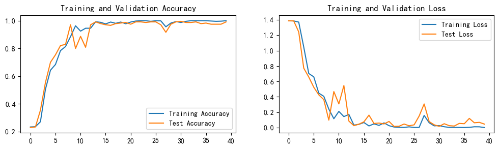
In [31]:
import matplotlib.pyplot as plt
#隐藏警告
import warnings
warnings.filterwarnings("ignore")               #忽略警告信息
plt.rcParams['font.sans-serif']    = ['SimHei'] # 用来正常显示中文标签
plt.rcParams['axes.unicode_minus'] = False      # 用来正常显示负号
plt.rcParams['figure.dpi']         = 100        #分辨率

epochs_range = range(epochs)

plt.figure(figsize=(12, 3))
plt.subplot(1, 2, 1)

plt.plot(epochs_range, train_acc, label='Training Accuracy')
plt.plot(epochs_range, test_acc, label='Test Accuracy')
plt.legend(loc='lower right')
plt.title('Training and Validation Accuracy')

plt.subplot(1, 2, 2)
plt.plot(epochs_range, train_loss, label='Training Loss')
plt.plot(epochs_range, test_loss, label='Test Loss')
plt.legend(loc='upper right')
plt.title('Training and Validation Loss')
plt.show()
2、指定图片进行预测
In [13]:
from PIL import Image

classes = list(train_dataset.class_to_idx)

def predict_one_image(image_path, model, transform, classes):

    test_img = Image.open(image_path).convert('RGB')
    plt.imshow(test_img)  # 展示预测的图片

    test_img = transform(test_img)
    img = test_img.to(device).unsqueeze(0)

    model.eval()
    output = model(img)

    _,pred = torch.max(output,1)
    pred_class = classes[pred]
    print(f'预测结果是:{pred_class}')
In [14]:
# 预测训练集中的某张照片
predict_one_image(image_path='E:/jupyter-notebook/data/6-data/Angelina Jolie/001_fe3347c0.jpg',
                  model=model,
                  transform=train_transforms,
                  classes=classes)
预测结果是:nike
3、模型评估
In [58]:
best_model.eval()
epoch_test_acc, epoch_test_loss = test(test_dl, best_model, loss_fn)
epoch_test_acc, epoch_test_loss
Out[58]:
(0.21944444444444444, 2.4482046564420066)
In [59]:
# 查看是否与我们记录的最高准确率一致
epoch_test_acc
Out[59]:
0.21944444444444444
原文地址:http://www.cnblogs.com/cauwj/p/16881415.html
1. 本站所有资源来源于用户上传和网络,如有侵权请邮件联系站长!
2. 分享目的仅供大家学习和交流,请务用于商业用途!
3. 如果你也有好源码或者教程,可以到用户中心发布,分享有积分奖励和额外收入!
4. 本站提供的源码、模板、插件等等其他资源,都不包含技术服务请大家谅解!
5. 如有链接无法下载、失效或广告,请联系管理员处理!
6. 本站资源售价只是赞助,收取费用仅维持本站的日常运营所需!
7. 如遇到加密压缩包,默认解压密码为"gltf",如遇到无法解压的请联系管理员!
8. 因为资源和程序源码均为可复制品,所以不支持任何理由的退款兑现,请斟酌后支付下载
声明:如果标题没有注明"已测试"或者"测试可用"等字样的资源源码均未经过站长测试.特别注意没有标注的源码不保证任何可用性