
# Human Motion Prediction Using Manifold-Aware Wasserstein GAN #paper
1. paper-info
1.1 Metadata
- Author:: [[Baptiste Chopin]], [[Naima Otberdout]], [[Mohamed Daoudi]], [[Angela Bartolo]]
- 作者机构::
- Keywords:: #HMP , #GAN
- Journal:: #IEEE
- Date:: [[2021-07-16]]
- 状态:: #Done
- 链接::http://arxiv.org/abs/2105.08715
- 修改时间:: 2022.11.22
1.2. Abstract
Human motion prediction aims to forecast future human poses given a prior pose sequence. The discontinuity of the predicted motion and the performance deterioration in long-term horizons are still the main challenges encountered in current literature. In this work, we tackle these issues by using a compact manifold-valued representation of human motion. Specifically, we model the temporal evolution of the 3D human poses as trajectory, what allows us to map human motions to single points on a sphere manifold. To learn these non-Euclidean representations, we build a manifold-aware Wasserstein generative adversarial model that captures the temporal and spatial dependencies of human motion through different losses. Extensive experiments show that our approach outperforms the state-of-the-art on CMU MoCap and Human 3.6M datasets. Our qualitative results show the smoothness of the predicted motions.
2. Introduction
- 领域:human motion prediction
- 问题:时间维度,如何使得预测的动作序列更加顺滑?空间维度,预测的动作更加真实?
- 之前的方法:RNN-based、CNN-based、GNN-based
- 作者的方法:
- 将人体动作当做轨迹,并且将这些轨迹映射到流行的单个紧凑点。能够使动作序列更加smoothness。
- 由于传统的GNN无法处理流式数据,于是作者提出了
a manifold-aware Wasserstein Generative Adversaial Network(WGAN) - 提出了多种损失函数来优化该网络,因为GAN很难train。
3. Methods
人体结构表示: 3D坐标
\(P_t=[x_1(t),y_1(t),z_1(t),…,x_k(t),y_k(t),z_k(t)]\): 某一时刻的姿势表示。
\(k\): 关节点数。
\(t\): 时刻
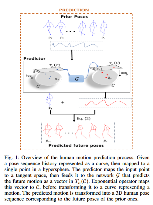
作者沿用[2],将人体骨架序列看做每个关节点的轨迹,从而将人体动作预测问题看做:给定一定序列的连续帧,去预测下一帧的点对应的曲线。将曲线描述为\(\alpha(t)\) ,问题变为:给定\(\alpha(t)_{t=1,,,\tau}\),预测\(\alpha(t)_{t=\tau+1,,,T}\)
为了能够更好的学习和建模\(\alpha(t)\),作者采用了square-root velocity function[1],该方法能够将曲线映射到一个超球面,得到一个超平面内的点(不同行为标签对应的轨迹产生的点之间的距离是不同的)。该方法的定义如下:
\(||.||\)操作表示为欧几里得2范数。
该方法在已知\(\alpha(0)\)的情况下,可以通过以下function还原\(\alpha(t)\):
为了更好的处理,将这个超球面的半径设置为1.
\(\mathcal{C}=\{q: \mathcal{I}->\mathcal{R}^n| ||q||=1\} \subset \mathcal{L}^2(\mathcal{I}, \mathcal{R}^n)\) :表示一个动作在超球面的映射。
由于该超空间不同于欧式空间,传统的GNN方法不能够处理该类数据,于是作者提出了新的GNN–PredictiveMA-WGAN
3.1 Network Architecture
PredictiveMA-WGAN由一个predictor\(\mathcal{G}\) 和discriminator\(\mathcal{D}\) 组成,对抗式学习。
During the training of these networks, we iteratively map the SRVF data back and forth to the tangent space using the exponential and the logarithm maps, defined in a particular point on the hypersphere.
在训练阶段,使用在超球面上的特定点中定义的指数和对数映射,以迭代的方式将SRVF数据来回映射到切线空间,然后输入到网络中。
\(\mathcal{G}\) :
36864输出通道的全连接层。
5个上采样块(512, 256,128,64,1),上采样块由nearest-neighbor upsampling跟着一个卷积块(3×3, stride 1)和ReLU function 构成。
\(\mathcal{D}\):
3个下采样块(64,32,16输出通道)
Conv layer(3×3 stride 1)
batch normalization
ReLU
3.2 Loss Function
- Adverasrial loss
- Reconstruction loss
- Skeleton integrity loss
这里解释没有看懂,具体看论文。
- Bone length loss
- Bone Length loss
Global loss
4. Experiments
- dataset
- Human3.6m
- CMU Motion Capture
- metric
- MPJPE
总结
与[2]的思路大致一致,将人体动作序列看过关节点的轨迹,在[2]中,利用DCT编码处理得到轨迹特征,然后利用GCN处理空间信息,在本文中,作者利用Square Root Velocity Function[1]将轨迹mapping 到一个超球体内,一条轨迹对应一点,然后将这些点投影到超球体的切线空间中,得到GAN网络模型的输入,最后训练GAN得到输出。
reference
[1] A. Srivastava, E. Klassen, S. H. Joshi and I. H. Jermyn, “Shape Analysis of Elastic Curves in Euclidean Spaces,” in IEEE Transactions on Pattern Analysis and Machine Intelligence, vol. 33, no. 7, pp. 1415-1428, July 2011, doi: 10.1109/TPAMI.2010.184.
[2]Mao W, Liu M, Salzmann M, et al. Learning trajectory dependencies for human motion prediction[C]//Proceedings of the IEEE/CVF International Conference on Computer Vision. 2019: 9489-9497.
原文地址:http://www.cnblogs.com/guixu/p/16922209.html