
-
使用tushare包获取某股票的历史行情数据。
-
输出该股票所有收盘比开盘上涨3%以上的日期。
-
输出该股票所有开盘比前日收盘跌幅超过2%的日期。
-
假如我从2010年1月1日开始,每月第一个交易日买入1手股票,每年最后一个交易日卖出所有股票,到今天为止,我的收益如何?
-
tushare:财经数据接口包(免费开源给金融分析人员提供)
-
pip install tushare
-
1、获取某只股票的历史行情数据在tushare官方文档看
import tushare as ts import pandas as pd from pandas import DataFrame,Series import numpy as np
#code:字符串形式的股票代码 df = ts.get_k_data(code='600519',start='2000-01-01') # 此接口不维护了 df
           date     open       close        high         low      volume    code
0   2001-08-27  -113.034    -112.849    -112.453    -113.329    406318.00   600519
1   2001-08-28  -112.949    -112.616    -112.591    -113.016    129647.79   600519
2   2001-08-29  -112.595    -112.702    -112.591    -112.751    53252.75    600519
3   2001-08-30  -112.719    -112.574    -112.501    -112.769    48013.06    600519
4   2001-08-31  -112.565    -112.590    -112.481    -112.627    23231.48    600519
... ... ... ... ... ... ... ...
5074    2022-11-16  1581.000    1585.250    1598.000    1568.000    26848.00    600519
5075    2022-11-17  1590.500    1567.000    1596.300    1552.880    30580.00    600519
5076    2022-11-18  1576.000    1567.130    1584.000    1556.000    23609.00    600519
5077    2022-11-21  1541.350    1519.980    1541.350    1498.530    39096.00    600519
5078    2022-11-22  1517.440    1539.950    1559.740    1516.110    29901.00    600519
5079 rows × 7 columns
#将互联网上获取的股票数据存储到本地(当前目录下) df.to_csv('./maotai1.csv')#调用to_xxx方法将df中的数据写入到本地进行存储 #将本地存储的数据读入到df df = pd.read_csv('./maotai1.csv') df.head()
Unnamed: 0  date    open    close   high    low volume  code
0   0   2001-08-27  -113.034    -112.849    -112.453    -113.329    406318.00   600519
1   1   2001-08-28  -112.949    -112.616    -112.591    -113.016    129647.79   600519
2   2   2001-08-29  -112.595    -112.702    -112.591    -112.751    53252.75    600519
3   3   2001-08-30  -112.719    -112.574    -112.501    -112.769    48013.06    600519
4   4   2001-08-31  -112.565    -112.590    -112.481    -112.627    23231.48    600519
#需要对读取出来的数据进行相关的处理
#删除df中指定的一列(Unnamed: 0 这一列 axis=1 drop是列)
df.drop(labels='Unnamed: 0',axis=1,inplace=True)
#查看每一列的数据类型 date列是字符串
df.info()
<class 'pandas.core.frame.DataFrame'>
RangeIndex: 5079 entries, 0 to 5078
Data columns (total 7 columns):
 #   Column  Non-Null Count  Dtype
---  ------  --------------  -----
 0   date    5079 non-null   object
 1   open    5079 non-null   float64
 2   close   5079 non-null   float64
 3   high    5079 non-null   float64
 4   low     5079 non-null   float64
 5   volume  5079 non-null   float64
 6   code    5079 non-null   int64
dtypes: float64(5), int64(1), object(1)
memory usage: 277.9+ KB
#将date列转为时间序列类型
df['date'] = pd.to_datetime(df['date'])
df.info()
<class 'pandas.core.frame.DataFrame'>
RangeIndex: 5079 entries, 0 to 5078
Data columns (total 7 columns):
 #   Column  Non-Null Count  Dtype
---  ------  --------------  -----
 0   date    5079 non-null   datetime64[ns]
 1   open    5079 non-null   float64
 2   close   5079 non-null   float64
 3   high    5079 non-null   float64
 4   low     5079 non-null   float64
 5   volume  5079 non-null   float64
 6   code    5079 non-null   int64
dtypes: datetime64[ns](1), float64(5), int64(1)
memory usage: 277.9 KB
#将date列作为源数据的行索引
df.set_index('date',inplace=True)
df.head()
                open    close           high         low       volume   code
date
2001-08-27  -113.034    -112.849    -112.453    -113.329    406318.00   600519
2001-08-28  -112.949    -112.616    -112.591    -113.016    129647.79   600519
2001-08-29  -112.595    -112.702    -112.591    -112.751    53252.75    600519
2001-08-30  -112.719    -112.574    -112.501    -112.769    48013.06    600519
2001-08-31  -112.565    -112.590    -112.481    -112.627    23231.48    600519
2、输出该股票所有收盘比开盘上涨3%以上的日期
#伪代码:(收盘-开盘)/开盘 > 0.03 (df['open'] - df['close']) / df['open'] > 0.03 #在分析的过程中如果产生了boolean值 则下一步马上将布尔值 作为源数据的 行索引 #如果布尔值作为df的行索引,则可以取出true对应的行数据,忽略false对应的行数据 df.loc[(df['open'] - df['close']) / df['open'] > 0.03] #获取了True对应的行数据(满足需求的行数据) df.loc[(df['open'] - df['close']) / df['open'] > 0.03].index #df的行数据


DatetimeIndex(['2006-05-29', '2006-11-14', '2006-11-30', '2006-12-11',
               '2006-12-14', '2006-12-18', '2006-12-29', '2007-01-09',
               '2007-01-11', '2007-01-12',
               ...
               '2021-08-26', '2021-10-18', '2021-12-29', '2022-01-13',
               '2022-01-28', '2022-03-07', '2022-10-10', '2022-10-19',
               '2022-10-24', '2022-10-27'],
              dtype='datetime64[ns]', name='date', length=819, freq=None)
View Code
3、输出该股票所有开盘比前日收盘跌幅超过2%的日期
#伪代码:(开盘-前日收盘)/前日收盘 < -0.02 () (df['open'] - df['close'].shift(1))/df['close'].shift(1) < -0.02 #将布尔值作为源数据的行索引取出True对应的行数据 df.loc[(df['open'] - df['close'].shift(1))/df['close'].shift(1) < -0.02] df.loc[(df['open'] - df['close'].shift(1))/df['close'].shift(1) < -0.02].index
DatetimeIndex(['2006-04-17', '2006-04-18', '2006-04-19', '2006-04-20',
               '2006-05-25', '2006-05-30', '2007-01-04', '2007-02-16',
               '2007-03-01', '2007-03-07',
               ...
               '2021-02-26', '2021-03-04', '2021-04-28', '2021-08-20',
               '2021-11-01', '2022-03-14', '2022-03-15', '2022-03-28',
               '2022-10-13', '2022-10-24'],
              dtype='datetime64[ns]', name='date', length=451, freq=None)
View Code
4、需求:假如我从2010年1月1日开始,每月第一个交易日买入1手股票,每年最后一个交易日卖出所有股票,到今天为止,我的收益如何?
分析:
-
时间节点:2010-2020
-
一手股票:100支股票
-
买:
-
一个完整的年需要买入1200支股票
-
-
卖:
-
一个完整的年需要卖出1200支股票
-
-
买卖股票的单价:
-
开盘价
-
new_df = df['2010-01':'2020-02']
new_df
new_df.head(2)
               open    close    high    low     volume  code
date
2010-01-04  109.760 108.446 109.760 108.044 44304.88    600519
2010-01-05  109.116 108.127 109.441 107.846 31513.18    600519
View Code
#买股票操作:首先找每个月的第一个交易日对应的行数据(捕获到开盘价)==》每月的第一行数据 #根据月份从原始数据中提取指定的数据resample('M') #first()每月第一个交易日对应的行数据 df_monthly = new_df.resample('M').first()#resample数据的重新取样 M根据月份 df_monthly #买入股票花费的总金额 cost = df_monthly['open'].sum()*100 cost
4010206.1
#卖出股票到手的钱
#特殊情况:当前时间是2020年 2020年买入的股票卖不出去
new_df.resample('A').last()
#将2020年最后一行切出去取数据到2019年
df_yearly = new_df.resample('A').last()[:-1]
df_yearly
               open   close  high    low    volume  code
date
2010-12-31  117.103 118.469 118.701 116.620 46084.0 600519
2011-12-31  138.039 138.468 139.600 136.105 29460.0 600519
2012-12-31  155.208 152.087 156.292 150.144 51914.0 600519
2013-12-31  93.188  96.480  97.179  92.061  57546.0 600519
2014-12-31  157.642 161.056 161.379 157.132 46269.0 600519
2015-12-31  207.487 207.458 208.704 207.106 19673.0 600519
2016-12-31  317.239 324.563 325.670 317.239 34687.0 600519
2017-12-31  707.948 687.725 716.329 681.918 76038.0 600519
2018-12-31  563.300 590.010 596.400 560.000 63678.0 600519
2019-12-31  1183.000 1183.000 1188.000 1176.510 22588.0 600519
View Code
#卖出股票到手的钱
resv = df_yearly['open'].sum()*1200
resv
4368184.8
#最后手中剩余的股票需要估量其价值计算到总收益中
#使用昨天的收盘价作为剩余股票的单价
last_monry = 200*new_df['close'][-1]
#计算总收益
resv+last_monry-cost
574778.6999999997
需求:双均线策略制定
1、使用tushare包获取某股票的历史行情数据
# 读取茅台股票数据,并删除无用数据列Unnamed: 0
df = pd.read_csv('./maotai.csv').drop(labels='Unnamed: 0',axis=1)
df
    date            open       close        high         low      volume    code
0   2001-08-27  -113.034    -112.849    -112.453    -113.329    406318.00   600519
1   2001-08-28  -112.949    -112.616    -112.591    -113.016    129647.79   600519
2   2001-08-29  -112.595    -112.702    -112.591    -112.751    53252.75    600519
3   2001-08-30  -112.719    -112.574    -112.501    -112.769    48013.06    600519
4   2001-08-31  -112.565    -112.590    -112.481    -112.627    23231.48    600519
... ... ... ... ... ... ... ...
5076    2022-11-18  1576.000    1567.130    1584.000    1556.000    23609.00    600519
5077    2022-11-21  1541.350    1519.980    1541.350    1498.530    39096.00    600519
5078    2022-11-22  1517.440    1539.950    1559.740    1516.110    29901.00    600519
5079    2022-11-23  1528.000    1549.000    1557.000    1521.040    22177.00    600519
5080    2022-11-24  1559.000    1519.990    1568.880    1513.980    27687.00    600519
5081 rows × 7 columns
View Code
#将date列转为时间序列且将其作为源数据的行索引 df['date'] = pd.to_datetime(df['date']) df.set_index('date',inplace=True) df.head()
                open       close        high         low        volume   code
date
2001-08-27  -113.034    -112.849    -112.453    -113.329    406318.00   600519
2001-08-28  -112.949    -112.616    -112.591    -113.016    129647.79   600519
2001-08-29  -112.595    -112.702    -112.591    -112.751    53252.75    600519
2001-08-30  -112.719    -112.574    -112.501    -112.769    48013.06    600519
2001-08-31  -112.565    -112.590    -112.481    -112.627    23231.48    600519
View Code
2、计算该股票历史数据的5日均线和30日均线
-
什么是均线?
-
对于每一个交易日,都可以计算出前N天的移动平均值,然后把这些移动平均值连起来,成为一条线,就叫做N日移动平均线。移动平均线常用线有5天、10天、30天、60天、120天和240天的指标。
-
5天和10天的是短线操作的参照指标,称做日均线指标;
-
30天和60天的是中期均线指标,称做季均线指标;
-
120天和240天的是长期均线指标,称做年均线指标。
-
-
-
均线计算方法:MA=(C1+C2+C3+…+Cn)/N C:某日收盘价 N:移动平均周期(天数)
# 取close列 rolling(5)把每五天取值mean()取均值 ma5 = df['close'].rolling(5).mean() # 30日均线 ma30 = df['close'].rolling(30).mean()
ma5 date 2001-08-27 NaN 2001-08-28 NaN 2001-08-29 NaN 2001-08-30 NaN 2001-08-31 -112.6662 ... 2022-11-18 1568.0760 2022-11-21 1565.4720 2022-11-22 1555.8620 2022-11-23 1548.6120 2022-11-24 1539.2100 Name: close, Length: 5081, dtype: float64 ma30 date 2001-08-27 NaN 2001-08-28 NaN 2001-08-29 NaN 2001-08-30 NaN 2001-08-31 NaN ... 2022-11-18 1561.499667 2022-11-21 1552.632333 2022-11-22 1544.631000 2022-11-23 1537.597667 2022-11-24 1531.597667 Name: close, Length: 5081, dtype: float64
View Code
# 将均线画出
import matplotlib.pyplot as plt
%matplotlib inline
# 画线
plt.plot(ma5[50:180])
plt.plot(ma30[50:180])

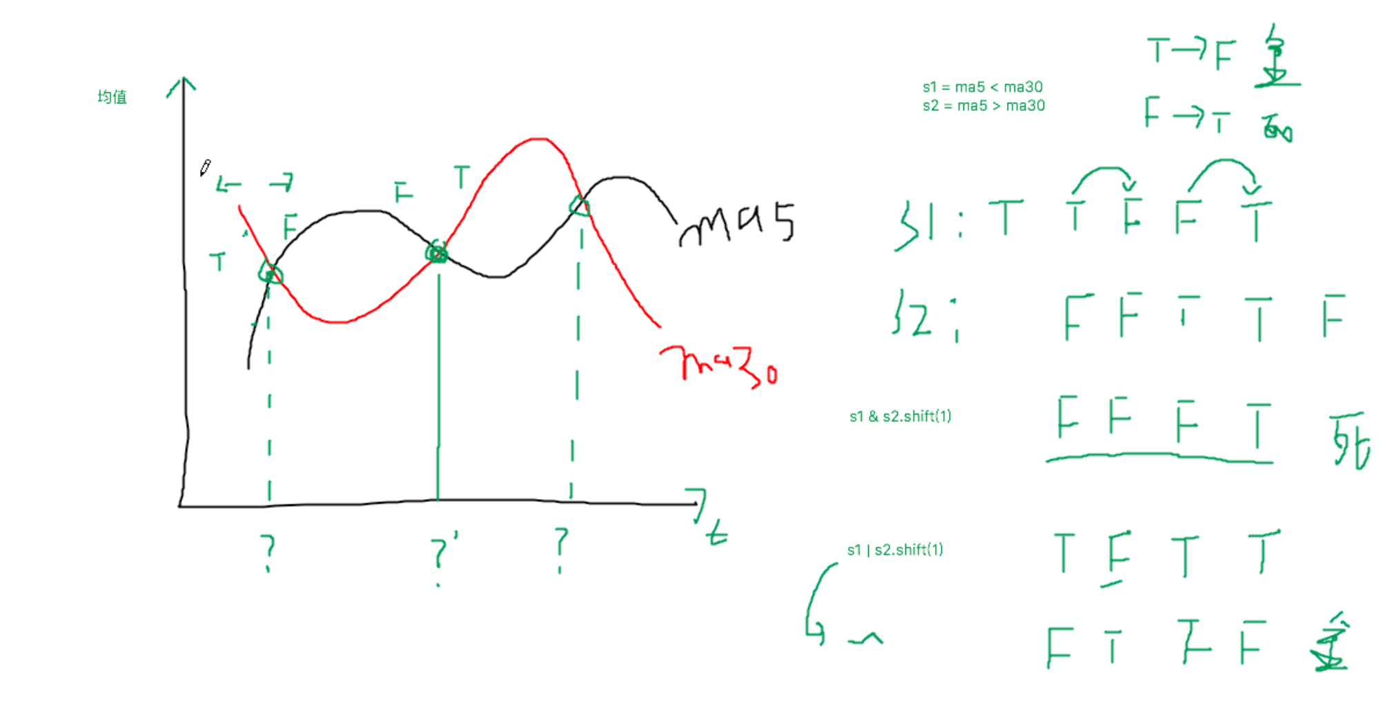
3、分析输出所有金叉日期和死叉日期
-
股票分析技术中的金叉和死叉,可以简单解释为:
-
分析指标中的两根线,一根为短时间内的指标线,另一根为较长时间的指标线。
-
如果短时间的指标线方向拐头向上,并且穿过了较长时间的指标线,这种状态叫“金叉”;
-
如果短时间的指标线方向拐头向下,并且穿过了较长时间的指标线,这种状态叫“死叉”;
-
一般情况下,出现金叉后,操作趋向买入;死叉则趋向卖出。当然,金叉和死叉只是分析指标之一,要和其他很多指标配合使用,才能增加操作的准确性。
-
# ma5 均值就是y轴 ma5 = ma5[30:] ma30 = ma30[30:] s1 = ma5 < ma30 s2 = ma5 > ma30 s1 # true代表ma5 < ma30
date
2001-10-15     True
2001-10-16     True
2001-10-17     True
2001-10-18     True
2001-10-19     True
              ...
2022-11-18    False
2022-11-21    False
2022-11-22    False
2022-11-23    False
2022-11-24    False
Name: close, Length: 5051, dtype: bool
View Code
df = df[30:] # shift(1)往后移一位 death_ex = s1 & s2.shift(1) #判定死叉的条件 如图s1和s2后移动1位的布尔值进行逻辑运算 df.loc[death_ex] #死叉对应的行数据 death_date = df.loc[death_ex].index # 死叉对应时间 golden_ex = ~(s1 | s2.shift(1))#判定金叉的条件 golden_date = df.loc[golden_ex].index #金叉的时间
4、如果我从假如我从2010年1月1日开始,初始资金为100000元,金叉尽量买入,死叉全部卖出,则到今天为止,我的炒股收益率如何?
-
分析:
-
买卖股票的单价使用开盘价
-
买卖股票的时机
-
最终手里会有剩余的股票没有卖出去
-
会有。如果最后一天为金叉,则买入股票。估量剩余股票的价值计算到总收益。
-
剩余股票的单价就是用最后一天的收盘价。
-
-
-
s1 = Series(data=1,index=golden_date) #1作为金叉的标识
s2 = Series(data=0,index=death_date) #0作为死叉的标识
s1
date
2001-11-22    1
2002-01-24    1
2002-02-04    1
2002-06-21    1
2002-12-05    1
             ..
2021-11-23    1
2022-04-07    1
2022-06-02    1
2022-09-29    1
2022-11-18    1
Length: 108, dtype: int64
View Code
s = s1.append(s2) # 金叉和死叉交替 s = s.sort_index() #存储的是金叉和死叉对应的时间 s = s['2010':'2020']##存储的是金叉和死叉对应的时间 first_monry = 100000 #本金,不变 money = first_monry #可变的,买股票话的钱和卖股票收入的钱都从该变量中进行操作 hold = 0 #持有股票的数量(股数:100股=1手) for i in range(0,len(s)): #i表示的s这个Series中的隐式索引 #i = 0(死叉:卖) = 1(金叉:买) if s[i] == 1:#金叉的时间 #基于100000的本金尽可能多的去买入股票 #获取股票的单价(金叉时间对应的行数据中的开盘价) time = s.index[i] #金叉的时间 p = df.loc[time]['open'] #股票的单价 开盘价open hand_count = money // (p*100) #使用100000最多买入多少手股票 hold = hand_count * 100 # 多少支股票 money -= (hold * p) #将买股票话的钱从money中减去 else: #将买入的股票卖出去 #找出卖出股票的单价 death_time = s.index[i] p_death = df.loc[death_time]['open'] #卖股票的单价 money += (p_death * hold) #卖出的股票收入 加入到money hold = 0 #如何判定最后一天为金叉还是死叉 last_monry = hold * df['close'][-1] #剩余股票的价值 #总收益 money + last_monry - first_monry
1501254.9999999995
聚宽(这是个学习平台)
原文地址:http://www.cnblogs.com/erhuoyuan/p/16926346.html