3 Generative models for discrete data

3.1 Bayesian concept learning

The psychological research has shown that people can learn concepts from positive examples alone.

3.1.1 Prior

The prior is the mechanism by which background knowledge can be brought to bear on a problem. Without this, rapid learning (i.e., from small samples sizes) is impossible.

首先是将背景知识用于解决问题的机制。如果没有这一点，快速学习(即快速学习)(即从较小的样本量)是不可能的。

3.1.2 Posterior

The posterior is the likelihood times the prior, normalized.

In general, when we have enough data, the posterior \(p(h|\mathcal{D})\) becomes peaked on a single concept, namely the Maximum A Posteriori (MAP) estimate.

Where \(\hat{h}^{MAP} = {\rm argmax}_h p(h|\mathcal{D})\) is the posterior mode, and \(\delta\) is the Dirac measure defined by

Since the likelihood term depends exponentially on N, and the prior stays constant, as we get more and more data, the MAP estimate converges towards the maximum likelihood estimate or MLE:

3.2.3 Posterior predictive distribution

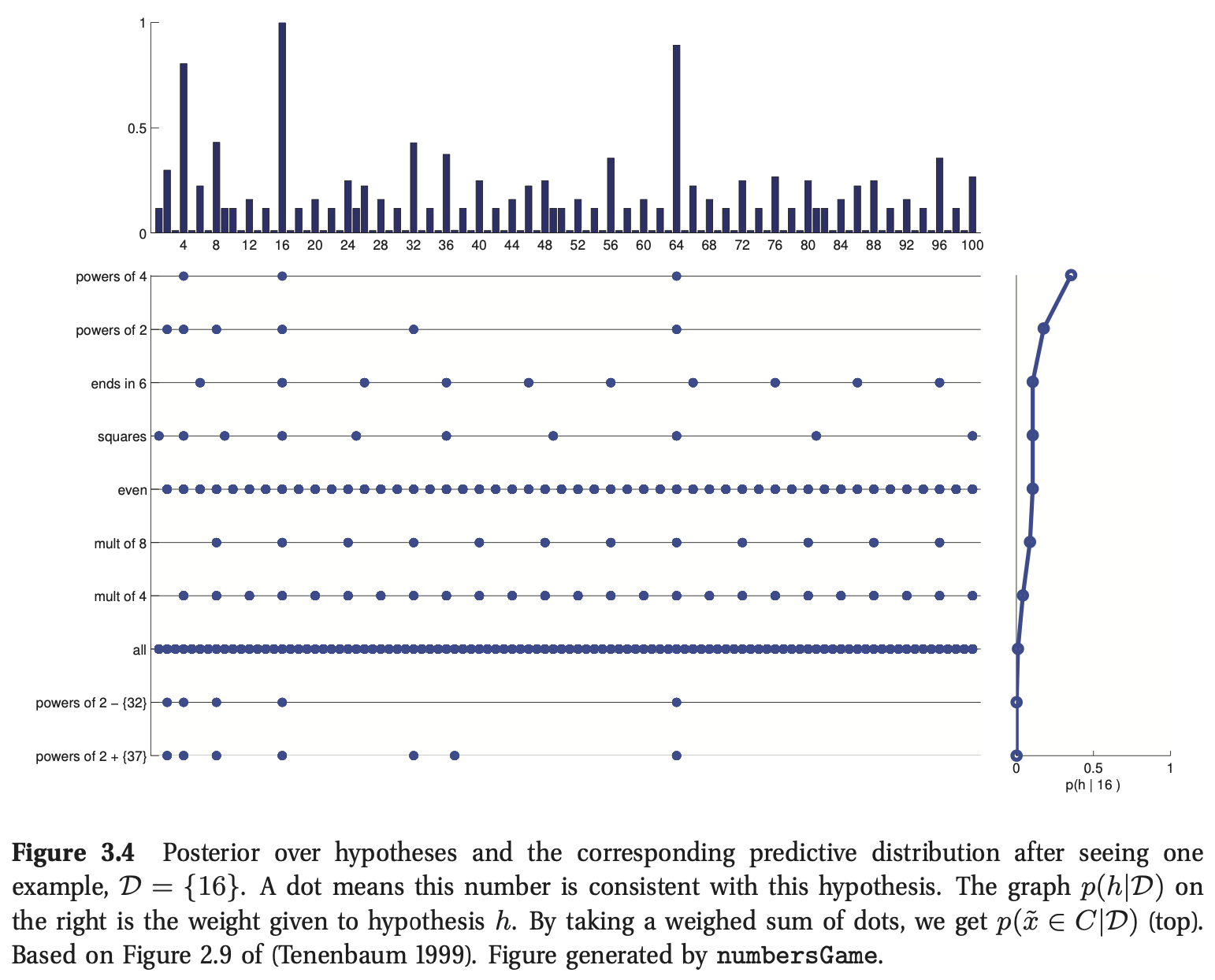
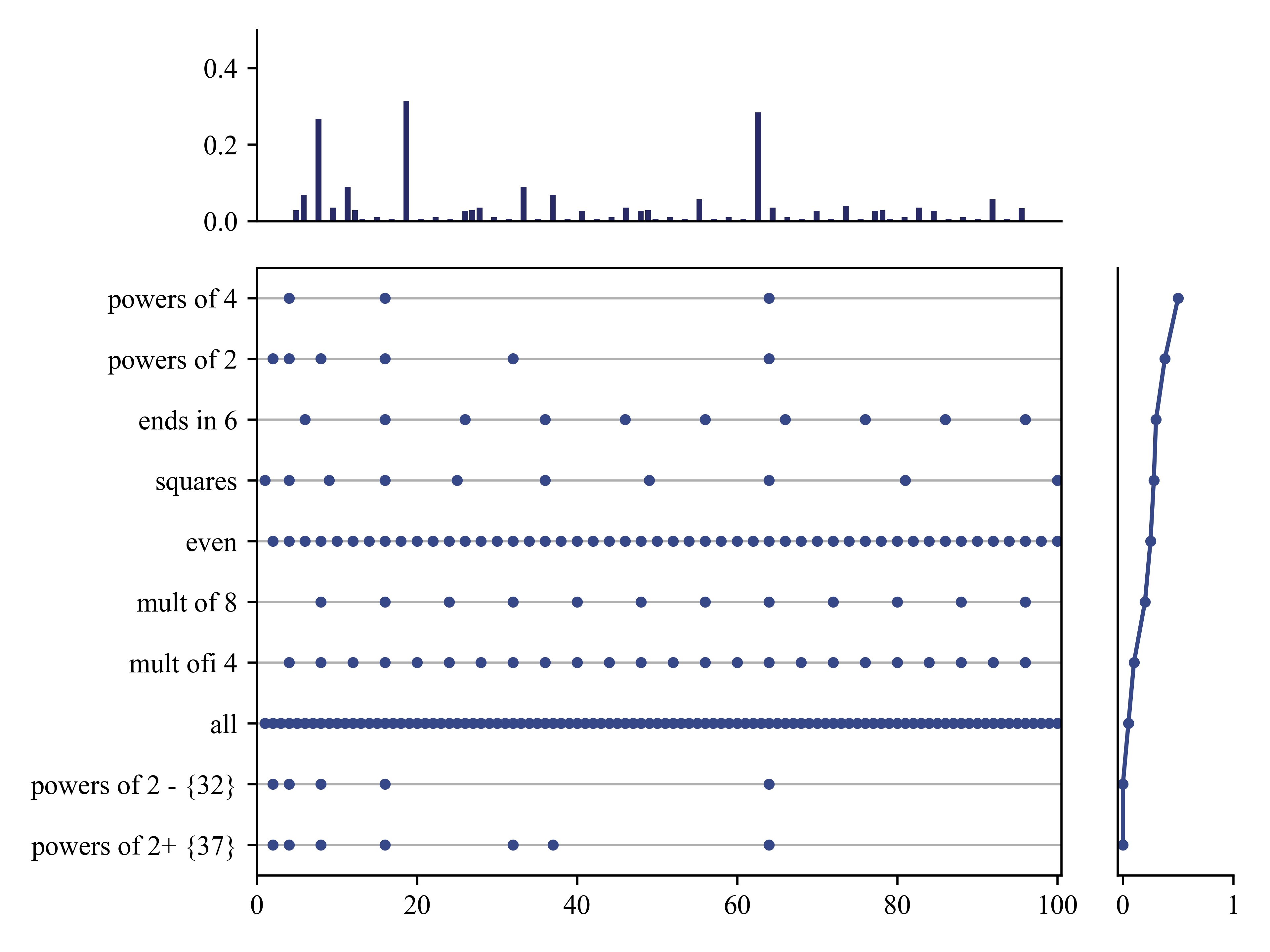
The posterior is our internal belief state about the world. The way to test if our beliefs are justified is to use them to predict objectively observable quantities (this is the basis of the scientific method). Specifically, the posterior predictive distribution is given by

This is just a weighted average of the predictions of each individual hypothesis and is called Bayes model averaging.

Python 实现原理

import numpy as np
import matplotlib.pyplot as plt
from matplotlib import gridspec

plt.rc('font', family='Times New Roman')

data = {'powers of 4': [4**(i+1) for i in range(3)], 'powers of 2': [2**(i+1) for i in range(6)], 'ends in 6': [6+i*10 for i in range(10)], 'squares': [(i+1)**2 for i in range(10)], 'even': [2*(i+1) for i in range(50)], 'mult of 8': [8*(i+1) for i in range(12)],'mult ofi 4': [4*(i+1) for i in range(24)], 'all': [i+1 for i in range(100)], 'powers of 2 - {32}': [2,4,8,16,64], 'powers of 2+ {37}': [2,4,8,16,32,37,64]}

gs = gridspec.GridSpec(15,12)
fig = plt.figure()
ax1 = plt.subplot(gs[0:4, 0:10])
ax2 = plt.subplot(gs[4:15, 0:10])
ax3 = plt.subplot(gs[4:15, 10:12])

plt.sca(ax2)
i=9
for key in data:

    plt.plot(data[key], [i for j in range(len(data[key]))],'.', color = '#374888')
    i-=1
plt.grid(linestyle='-', axis='y')
plt.axis([0,100.5,-0.5,9.5])
plt.yticks([i for i in range(10)],list(data.keys())[::-1])

plt.sca(ax3)
p_h = [0,0,0.05,0.1,0.2,0.25,0.28,0.3,0.38,0.5]
y_h = [i for i in range(10)]
plt.plot(p_h,y_h,'-',color='#374888')
plt.plot(p_h,y_h,'.',color='#374888')
plt.axis([-0.05,1,-0.5,9.5])
plt.yticks([])
ax3.spines['top'].set_visible(False)
ax3.spines['right'].set_visible(False)

plt.sca(ax1)
x_dist = np.arange(1,101,1)
y_pp = []
ph = p_h.reverse()
for i in range(len(x_dist)):
    y_pp_temp = 0
    j=0
    for key in data:
        if x_dist[i] in data[key]:
            y_pp_temp += 1/len(data[key])* (p_h[j])
        j+=1
    y_pp.append(y_pp_temp)
plt.bar(x_dist,y_pp, color='#282A65')
plt.xticks([])
plt.ylim([0,0.5])
ax1.spines['top'].set_visible(False)
ax1.spines['right'].set_visible(False)

plt.tight_layout()
plt.show()

When we have a small and/or ambiguous dataset, the posterior \(p(h|\mathcal{D})\) is vague, which induces a broad predictive distribution. However, once we have “figured things out”, the posterior becomes a delta function centered at the MAP estimate. In this case, the predictive distribution

This is called a plug-in approximation to the predictive density and is very widely used, due to its simplicity.

3.2 The beta-binomial model

3.2.1 Likelihood

Suppose \(X_i \sim {\rm Ber}(\theta)\), where \(X_i={1,0}\) and \(\theta \in [0,1]\) is the rate parameter. If the data are iid, the likelihood has the form

Where we have \(N_1 = \sum_{i=1}^N \mathbb{I}(x_i=1)\) and \(N_0 = \sum_{i=1}^N \mathbb{I}(x_i=0)\)

Suppose the data consists of the count of the number of \(N_1\) observed in a fixed number \(N = N_1 + N_0\) of trials. In this case, we have \(N_1 ∼ Bin(N, θ)\), where Bin represents the binomial distribution, which has the following pmf:

3.2.2 Prior

When the prior and the posterior have the same form, we say that the prior is a conjugate prior for the corresponding likelihood.

In the case of the Bernoulli, the conjugate prior is the beta distribution

The parameters of the prior are called hyper-parameters.

Beta Distribution

The beta distribution has support over the interval \([0, 1]\)

mean: \(\cfrac{a}{a+b}\), mode: \(\cfrac{a-1}{a+b-2}\), var: \(\cfrac{ab}{(a+b)^2(a+b+1)}\)

Where \(\Gamma(x)\) is the gamma function.

3.2.3 Posterior

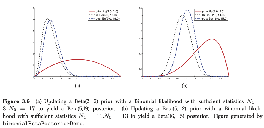
If we multiply the likelihood by the beta prior we get the following posterior:

Python 实现原理

import numpy as np
import matplotlib.pyplot as plt
from scipy import stats
plt.rc('font', family='Times New Roman')

x= np.linspace(0,1,100)
prior_Be = stats.beta(a=2,b=2).pdf(x)
# Ber -> N_1 = 3 , N2 = 17
likeli_Be = stats.beta(a=4,b=18).pdf(x)
posteri_Be = stats.beta(a=5,b=19).pdf(x)

prior_Be2 = stats.beta(a=5,b=2).pdf(x)
# Ber -> N_1 = 11 , N2 = 13
likeli_Be2 = stats.beta(a=12,b=14).pdf(x)
posteri_Be2 = stats.beta(a=16,b=15).pdf(x)

fig,ax = plt.subplots(1,2, figsize=(10,4),)

plt.sca(ax[0])
plt.plot(x,prior_Be, color='#C73834',label='prior Be(2,2)')
plt.plot(x,likeli_Be, 'k--', label='lik Be(4,18)')
plt.plot(x,posteri_Be,'-.', color='#374888', label='post Be(5,19)')
plt.legend()
ax[0].spines['top'].set_visible(False)
ax[0].spines['right'].set_visible(False)
plt.axis([0.01,1,0.01,6])

plt.sca(ax[1])
plt.plot(x,prior_Be2, color='#C73834',label='prior Be(5,2)')
plt.plot(x,likeli_Be2, 'k--', label='lik Be(12,14)')
plt.plot(x,posteri_Be2,'-.', color='#374888', label='post Be(16,15)')
plt.legend()
ax[1].spines['top'].set_visible(False)
ax[1].spines['right'].set_visible(False)
plt.axis([0.01,1,0.01,4.5])

plt.tight_layout()
plt.savefig('./Figure/3.6Beta-binomial分布.png', dpi=600)
plt.show()

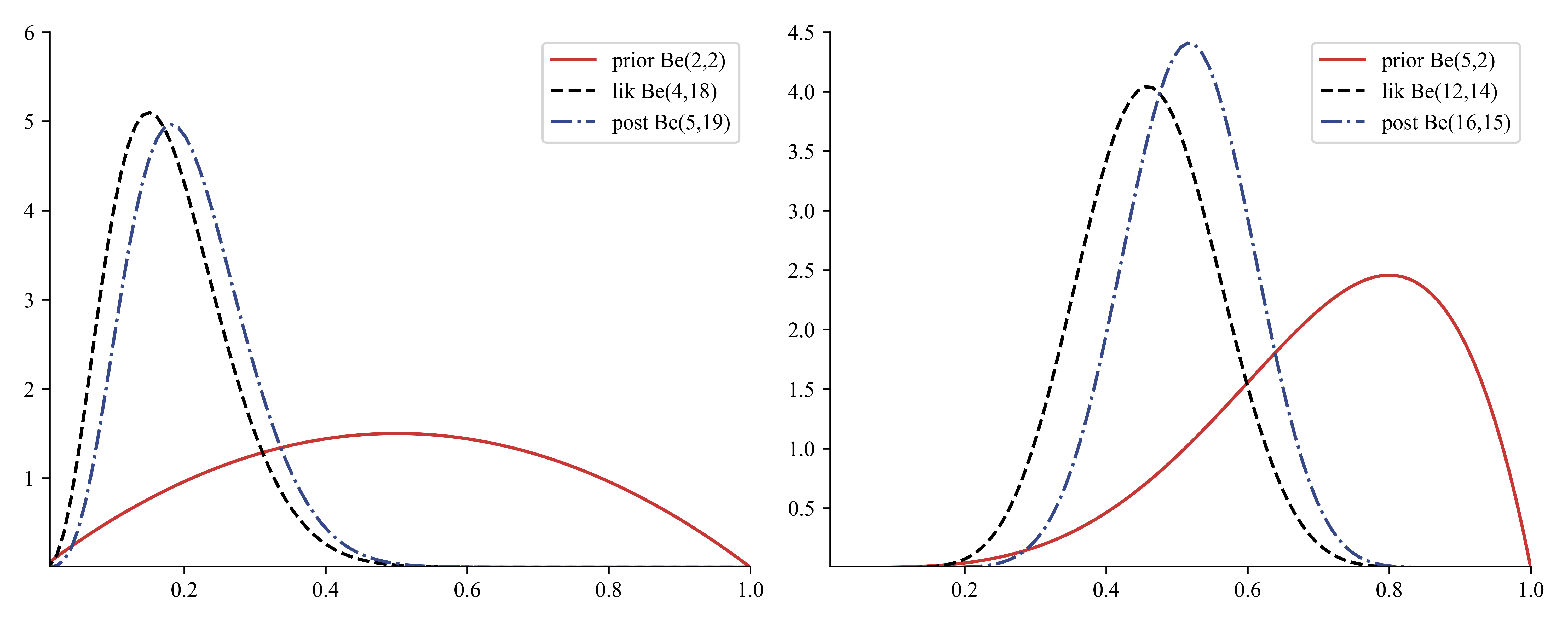
Updating the posterior sequentially is equivalent to updating in a single batch. Suppose we have two data sets \(\mathcal{D_a}\) and \(\mathcal{D_b}\) with sufficient statistics \(N_1^a\), \(N_0^a\) and \(N_1^b\) , \(N_0^b\) . Let \(N_1 = N_1^a + N_1^b\) and \(N_0 = N_0^a + N_0^b\) be the sufficient statistics of the combined datasets. In batch mode we have

In sequential mode, we have

3.2.3.1 Posterior mean and mode

The MAP estimate is given by

If we use a uniform prior, then the MAP estimate reduces to the MLE, which is just the empirical fraction of heads:

The posterior mean is given by,

Let \(\alpha_0 = a+b\), the posterior mean is given by

where \(\lambda = \cfrac{\alpha_0}{N+\alpha_0}\) is the ratio of the prior to posterior equivalent sample size. The weaker the prior, the smaller is \(λ\), and hence the closer the posterior mean is to the MLE.

3.2.3.2 Posterior variance

The variance of the Beta posterior is given by

We can simplify this formidable expression in the case that \(N ≫ a, b\), to get

where \(\hat{\theta}\) is the MLE. Hence the “error bar” in our estimate (i.e., the posterior standard deviation), is given by

3.2.4 Posterior predictive distribution

Consider predicting the probability of heads in a single future trial under a \({\rm Beta}(a, b)\) posterior. We have

The mean of the posterior predictive distribution is equivalent (in this case) to plugging in the posterior mean parameters: \(p(\widetilde{x}|\mathcal{D}) = {\rm Ber}(\widetilde{x}|\mathbb{E}[\theta|\mathcal{D}])\)

3.2.4.1 Overfitting and the black swan paradox

Suppose instead that we plug-in the \(MLE\), i.e., we use \(p(\widetilde{x}|\mathcal{D}) ≈ {\rm Ber}(\widetilde{x}|\hat{\theta}_{MLE})\). Unfortunately, this approximation can perform quite poorly when the sample size is small. This is called the zero count problem or the sparse data problem, and frequently occurs when estimating counts from small amounts of data.

The zero-count problem is analogous to a problem in philosophy called the black swan paradox.

举个栗子：

假定我们使用均匀分布作为先验，那么在先验的Beta分布中， \(a=b=1\)，在这种情况下，插入后验平均值给出了拉普拉斯的继承规则（Laplace’s rule of succession）

This justifies the common practice of adding 1 to the empirical counts, normalizing and then plugging them in, a technique known as add-one smoothing.

Plugging in the MAP parameters would not have this smoothing effect, since the mode has the form \(\hat{\theta} = \cfrac{N_1+a-1}{N+a+b-2}\), which becomes the MLE if \(a=b=1\)

3.2.4.2 Predicting the outcome of multiple future trials

Suppose now we were interested in predicting the number of heads, \(x\), in \(M\) future trials. This is given by

We recognize the integral as the normalization constant for a \({\rm Beta}(a+x, M−x+b)\) distribution.

Thus we find that the posterior predictive is given by the following, known as the (compound) beta-binomial distribution:

This distribution has the following mean and variance

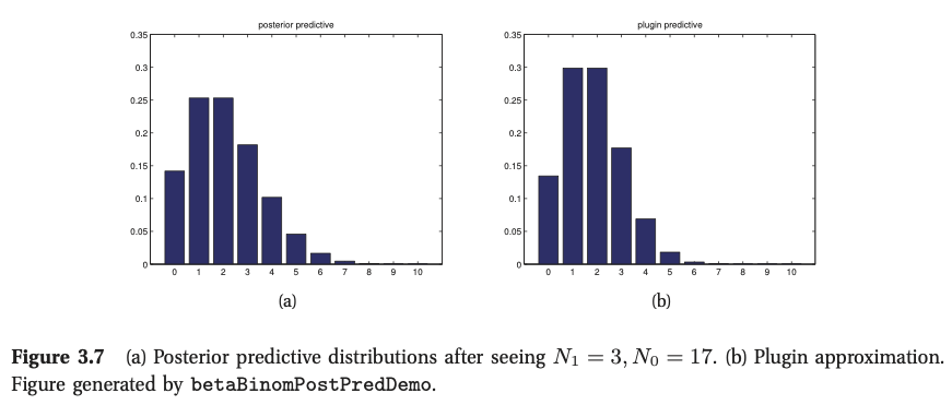
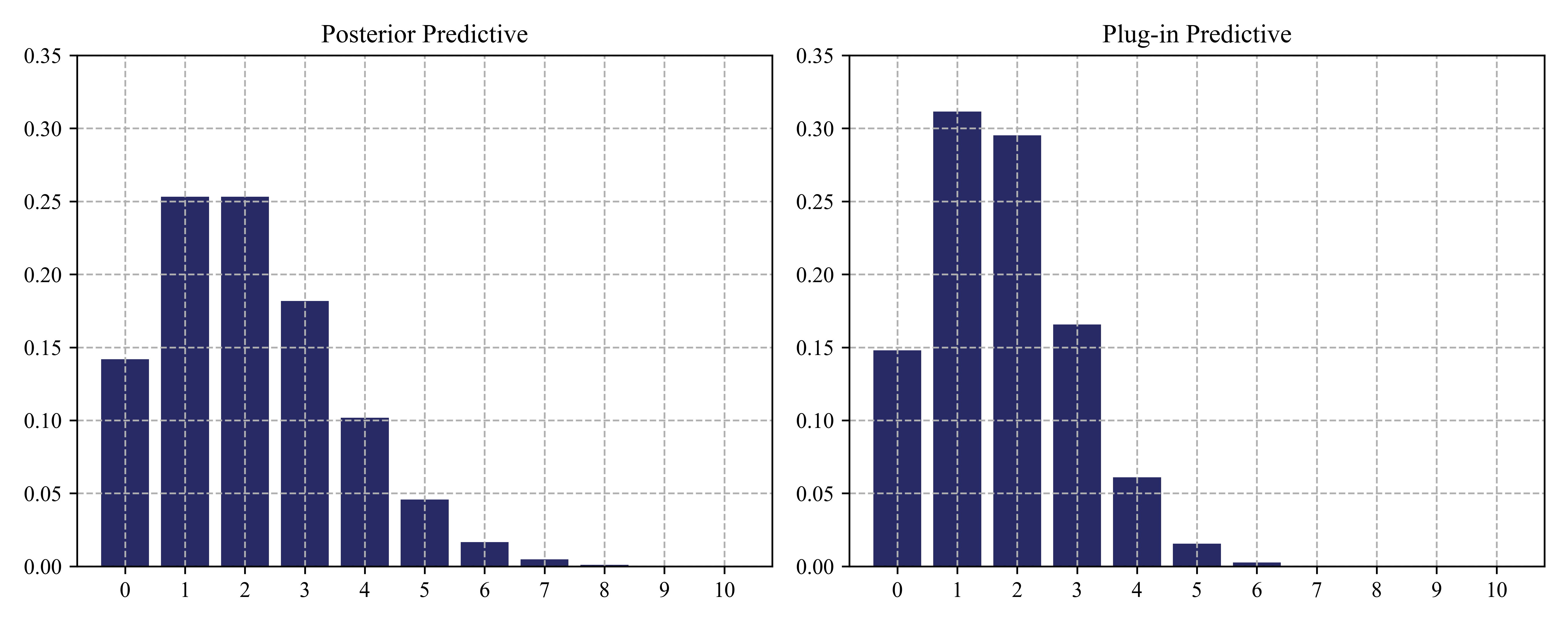
Given \(M=10\), we start with a \({\rm Beta}(2,2)\) prior, and (b) plot the posterior predictive density after seeing \(N_1 = 3\) heads and \(N_0 = 17\) tails. (b) plots a plug-in approximation using a MAP estimate. We see that the Bayesian prediction has longer tails, spreading its probablity mass more widely, and is therefore less prone to overfitting and blackswan type paradoxes.

Python 实现原理

import numpy as np
import matplotlib.pyplot as plt
from scipy import stats
plt.rc('font', family='Times New Roman')

'''
prior ~ Beta(2,2)
observation ~ N1=3 ,N0=17
p(\theta | D) ~ Beta(a+N1,b+N0) -> Beta(5,19)
'''
n, a, b = 10,5,19
x = np.arange(0,10,1)
ppd_1=stats.betabinom(n, a, b).pmf(x)

'''
\theta_MAP = \frac{a+N1-1}{a+b+N-2} = 4/23
x ~ Bin(n,theta)
'''
n, p= 10, 4/23
ppd_2 = stats.binom.pmf(x,n=n,p=p)

_, ax = plt.subplots(1,2,figsize=(10,4))

plt.sca(ax[0])
plt.bar(x, ppd_1, color='#282A65')
plt.axis([-0.8,10.8,0,0.35])
plt.xlabel('',fontsize=11)
plt.ylabel('',fontsize=11)
plt.title('Posterior Predictive', fontsize=12)
plt.grid(linestyle='--')
plt.xticks(np.arange(0,11,1))

plt.sca(ax[1])
plt.bar(x, ppd_2, color='#282A65')
plt.axis([-0.8,10.8,0,0.35])
plt.xlabel('',fontsize=11)
plt.ylabel('',fontsize=11)
plt.title('Plug-in Predictive', fontsize=12)
plt.grid(linestyle='--')
plt.xticks(np.arange(0,11,1))

plt.tight_layout()
plt.savefig('./Figure/3.7后验预测分布.png',dpi=600)
plt.show()

3.3 The Dirichlet- multinomial model

3.3.1 Likelihood

Suppose we observe \(N\) dicerte rolls, \(\mathcal{D} = \{x_1,…,x_N\}\), where \(x_i ∈ \{1,\ldots,K\}\). If we assume the data is iid, the likelihood has the form

Where \(N_k = \sum_{i=1}^N\mathbb{I}(y_i=k)\) is the number of times event k occured.

3.3.2 Prior

Since the parameter vector lives in the \(K\)-dimensional probability simplex, we need a prior that has support over this simplex. Ideally it would also be conjugate. Fortunately, the Dirichlet distribution satisfies both criteria. So we will use the following prior:

Dirichlet distribution

A multivariate generalization of the beta distribution is the Dirichlet distribution , which has support over the probability simplex,

where \(\alpha_0 \triangleq \sum_{k=1}^K \alpha_k\)

\(\mathbb{E}[x_k]=\cfrac{\alpha_k}{\alpha_0}\), \({\rm mode}[x_k] = \cfrac{\alpha_k-1}{\alpha_0-K}\), \({\rm var}[x_k] = \cfrac{\alpha_k(\alpha_0-\alpha_k)}{\alpha_0^2(\alpha_0+1)}\)

3.3.3 Posterior

Multiplying the likelihood by the prior, we find that the posterior is also Dirichlet:

We can derive the mode of this posterior (i.e., the MAP estimate) by using calculus. However, we must enforce the constraint that \(\sum_k\theta_k = 1.^2\). We can do this by using a Lagrange multiplier. The constrained objective function, or Lagrangian, is given by the log likelihood plus log prior plus the constraint:

To simplify notation, we define \(N_k^{‘} = \triangleq N_k+\alpha_k-1\), Taking derivatives with respect to \(λ\) yields the original constraint:

Taking derivatives with respect to \(θ_k\) yields

We can solve for \(λ\) using the sum-to-one constraint:

where \(\alpha_0 \triangleq \sum_{k=1}^{K}\alpha_k\) is the equivalent sample size of the prior. Thus the MAP estimate is given by

If we use a uniform prior, \(\alpha_k=1\), we recover the MLE:

3.3.4 Posterior predictive

The posterior predictive distribution for a single multinoulli trial is given by the following expression:

where \(\theta_{−j}\) are all the components of \(\boldsymbol{\theta}\) except \(θ_j\).

3.4 Naive Bayes classifiers

Specifing the class conditional distribution,\(p{(\mathbf{x}|y=c)}\). The simplest approach is to assume the features are conditionally independent given the class label. This allows us to write the class conditional density as a product of one dimensional densities:

Where \(\mathcal{D}\) is the number of features.

The resulting model is called a naive Bayes classifier (NBC). The model is called “naive” since we do not expect the features to be independent, even conditional on the class label.

The form of the class-conditional density depends on the type of each feature.

• In the case of real-valued features, we can use the Gaussian distribution: \(p(\mathbf{x}|y=c,\boldsymbol{\theta}) = \prod_{j=1}^D \mathcal{N}(x_j|\mu_{jc},\sigma^2_{jc})\), where \(\mu_{jc}\) is the mean of feature \(j\) in objects of class \(c\), and \(\sigma^2_{jc}\) is its variance.
• In the case of binary features, \(x_j=\{0,1\}\), we can use the Bernoulli distribution: \(p(\mathbf{x}|y=c,\boldsymbol{\theta}) = \prod_{j=1}^\mathcal{D}\mathrm{Ber}(x_j|\mu_{jc})\), where \(\mu_{jc}\) is the probability that feature \(j\) occurs in class \(c\). This is sometimes called the multivariate Bernoulli naive Bayes model.
• In the case of categorical features, \(x_j \in \{1,\ldots, K\}\), we can model use the multinoulli distribution: \(p(\mathbf{x}|y=c,\boldsymbol{\theta}) = \prod_{j=1}^{\mathcal{D}} \mathrm{Cat}(x_j|\mu_{jc})\), where \(\mu_{jc}\) is a histogram over the \(K\) possible values for \(x_j\) in class \(c\).

分类分布、Categorical 分布

3.4.1 Model fitting

3.4.1.1 MLE for NBC

The probability for a single data case is given by

Hence the log-likelihood is given by

We see that this expression decomposes into a series of terms, one concerning \(\textcolor{red}{π}\), and DC terms containing the \(θ_{jc}\)’s. Hence we can optimize all these parameters separately.

the MLE for the class prior is given by

where \(N_c \triangleq \sum_i \mathbb{I}(y_i=c)\) is the number of examples in class \(c\).

The MLE for the likelihood depends on the type of distribution we choose to use for each feature. For simplicity, let us suppose all features are binary, so \(x_j|y = c \sim \mathrm{Ber}(\theta_{jc})\), In this case, the MLE becomes

3.4.1.2 Bayesian navie Bayes

The trouble with maximum likelihood is that it can overfit. ==> \(\theta_{jc}=1\)

The anthor problem is that balck swan paradox. ==> \(p(y=c|\mathbf{x},\hat{\boldsymbol{\theta}})\)

A simple solution to overfitting is to be Bayesian. For simplicity, we will use a factored prior:

We will use a \(\mathrm{Dir}(\boldsymbol{\alpha})\) prior for \(π\) and a \(\mathrm{Beta}(β_0,β_1)\) prior for each \(\theta_{jc}\). Often we just take \(\boldsymbol{\alpha} = 1\) and \(\boldsymbol{\beta} = 1\), corresponding to add-one or Laplace smoothing.

3.4.2 Using the model for prediction

The correct Bayesian procedure is to integrate out the unknown parameters:

where \(\alpha_0 = \sum_{c}\alpha_c\)

If we have approximated the posterior by a single point, \(p(\boldsymbol{\theta}|\mathcal{D}) \approx \delta_{\hat{\boldsymbol{\theta}}}(\boldsymbol{\theta})\), where \(\hat{\boldsymbol{\theta}}\) may be the ML or MAP estimate, then the posterior predictive density is obtained by simply plugging in the parameters.

3.4.3 The log-sum-exp trick

The problem is that$ p(\mathbb{x}|y = c) $ is often a very small number, especially if \(\mathbf{x}\) is a high-dimensional vector. This is because we require that \(\sum_{\mathbf{x}} p(\mathbf{x}|y) = 1\), so the probability of observing any particular high-dimensional vector is small. The obvious solution is to take logs when applying Bayes rule.

We can’t add up in the log domain. Fortunately, we can factor out the largest term, and just represent the remaining numbers relative to that.

Where \(B=\max_cb_c\), This is called the log-sum-exp trick, and is widely used.

3.4.4 Feature selection using mutual information

Since an NBC is fitting a joint distribution over potentially many features, it can suffer from overfitting. In addition, the run-time cost is \(O(D)\), which may be too high for some applications. One common approach to tackling both of these problems is to perform feature selection. The simplest approach to feature selection is to evaluate the relevance of each feature separately, and then take the top K, where K is chosen based on some tradeoff between accuracy and complexity. This approach is known as variable ranking, filtering, or screening.

If the features are binary, the MI can be computed as follows

where \(\pi_c = p(y=c)\), \(\theta_{jc} = p(x_j=1|y=c)\), and \(\theta_j =p(x_j=1) = \sum_c\pi_c\theta_{jc}\)

原文地址：http://www.cnblogs.com/zhangjianhua0728/p/16928129.html